Chapter 1 General information on R & RStudio
software environment for statistical computing and graphics R is based on S
GPL (general public license) –> free software
R-1.0.0 was published in 2000; current version: R-4.2.0 (4.0.0 release soon)
R is available for several OS (including 64bit versions) functionality can be extended by packages
Packages are bundles of functions and data (and corresponding documentation)
Comprehensive R Archive Network (CRAN) is the primary source for packages: April 2013: 4,437 packages on CRAN; October 2014: 5,966 packages; September 2015: 7,084 packages; September 2016: 9,237 packages, April 2019: 14,030 packages
Wide dissemination in academia + private industry (see pdfs). Along with Python, R is the dominating data science software. For cases and illustrations, check out https://www.kaggle.com/ and https://www.r-bloggers.com/.
Advantages: flexibility (no separation between input and output), transparency (documentation and source code publicly available), extensibility (packages)
Disadvantages: performance (slow compared to C, Java, etc.), no quality checks of packages, sloppy syntax
Web page and further information: https://www.r-project.org/
List of literature: http://ftp5.gwdg.de/pub/misc/cran/other-docs.html
1.1 Using RStudio
1.1.1 Introduction
RStudio is a all-in-one front-end for R including a GUI, script editor, package management, and a lot more. Thus, RStudio is an IDE. RStudio can be obtained from https://www.rstudio.org for free. Note: You need to install R first.
Once installed, RStudio looks like this:
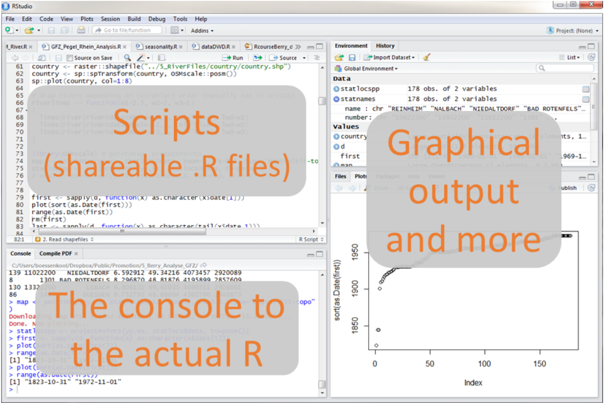
RStudio IDE
Write code in script files (File -> New File -> R Script). Execute code by pressing Ctrl + r (Cmd + r on MAc). Execution copies code chunks into the console where the command is processed. Save the script via ‘File -> Save as…’. Script files contain code and are the recipes to create objects, perform analysis etc. Note that scripts do not contain data objects. These are stored in workspaces (see below). Workspaces must be stored seperately-
1.1.2 Projects
RStudio offers projects to structure projects conducted with R. To create a project a project, select the dropdown menu on the upper right corner of the RStudio window (Project:
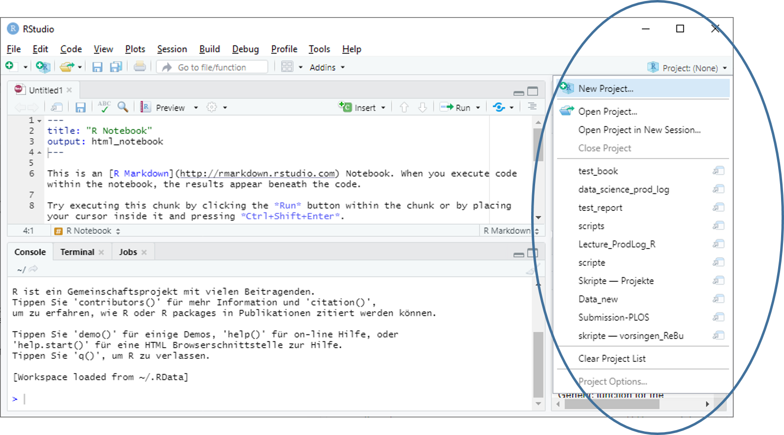
RStudio IDE
A dialog appears asking you what specific project is to be created. Select a simple project and subsequently a name and directory where to put the project-related files.
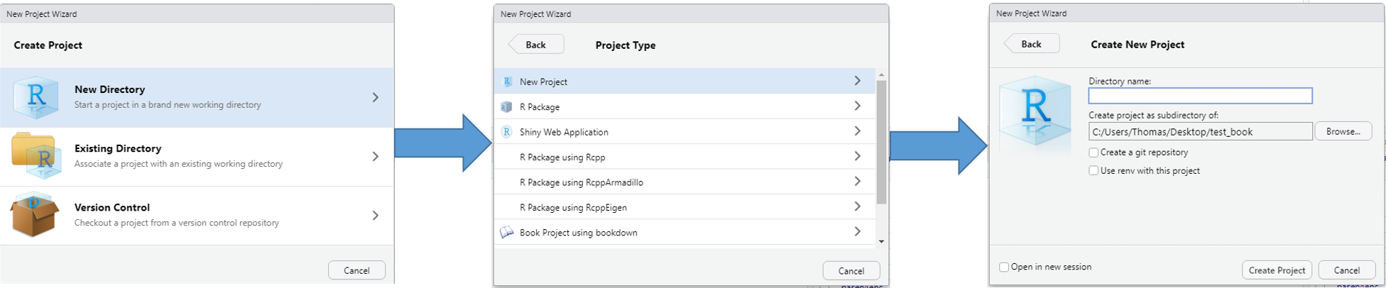
RStudio IDE
In this directory, automatically the workspace and scripts are saved which eases project management considerably. Additionally, once you open a project, workspace and script files are restored automatically.
1.1.3 Markdown
RStudio offers a wide range of auxiliary features for creating R-based projects. One particularly helpful feature is the implementation of Pandoc via Markdown (https://de.wikipedia.org/wiki/Markdown). This feature allows you to compile documents including R commands which are automatically embedded in html, pdf or epub documents. An encompassing introduction can be found here https://bookdown.org/yihui/rmarkdown/.
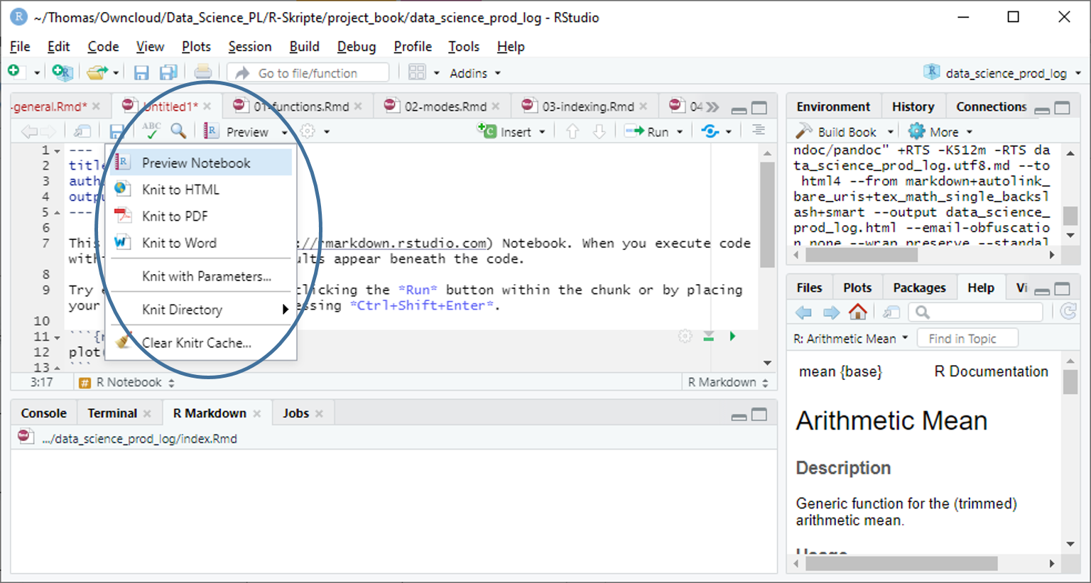
To create a markdown document, navigate to “File -> New File -> R Notebook” which creates the simplest possible document. To compile the document, select the dropdown menu of the “Preview” button right above the script file and ““knit” the desired document format:
For a cheat sheet on the most basic markdown commands, see https://github.com/adam-p/markdown-here/wiki/Markdown-Cheatsheet#links
1.2 Packages
Any user of R can distribute his/her code, functions, and data via a standardized procedure by bundling the content in packages. Packages are centrally stored on repository servers wordwide. To browse packages visit https://cran.r-project.org/. Before a package (and the corresponding functions and data) can be used, the package needs to be downloaded from CRAn once and afterwards loaded into the workspace, e.g.:
install.packages("robustbase") # download package robustbase
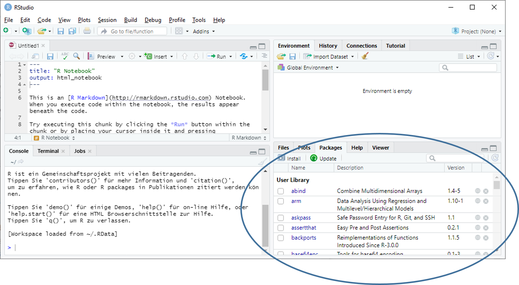
library(robustbase) # load package robustbaseAlternatively you can manage packages via right-left pane in RStudio
1.3 R as a simple calculator
5 + 5 # summation## [1] 105 * 5 # multiplication## [1] 255^0.5 # square root, decimal separator## [1] 2.2360685^.5## [1] 2.236068# note the difference:
5^(.5/2)## [1] 1.4953495^.5/2## [1] 1.1180341.4 Objects & workspace
Objects in R are of different types to numbers, vectors, matrices as well as functions. Creating an object is via <- or =. However, using ´=´ is considered bad style.
test <- 101         # assignment
102 -> test2        # not recommended
test3 = 103         # equality sign, not recommended
By creating objects these are in the workspace (see upper-right panel in RStudio). Workspaces can saved and loaded (Session -> Load Workspace / Save Workspace as).
Objects in the workspace can be listed and removed.
ls() # list all objects in workspace## [1] "test" "test2" "test3"rm(test3) # remove object test3The workspace is the global environment. Any chunks of code can work with objects in the workspace only.
test2 # show object test2
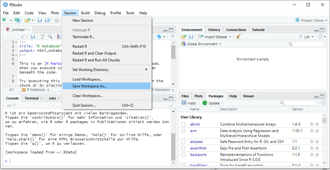
test3 # error as test3 has been removed from workspaceTo save a workspace use save.image("<file.name>") or navigate to “Session –> Save Workspace As …”