Chapter 3 Modes, types & classes of objects
Any object in R is of a particular type, is stored in a particular way, and belongs to a particular class. Types and storage modes describe how an object is handled in R, and object classes are based on how the objects can be used. The following table shows the functions which can be used to query class, mode and type of objects:
| Type | Mode | class |
|---|---|---|
| `typeof() | |
|
Note that in most text the distinction between data and object types, storage and classes is not clear and depends on the context. Usually, data types comprise vectors, matrices and so on.
3.1 Types & storage modes
An atomic object is usually called scalar. Typically, a scalar has one type of “logical”, “integer”, “double”, “complex”, “character”, “raw” and “list”, “closure”, or “builtin” (the latter two refer to functions). Here are some examples:
mode(x <- 5)                # the storage mode of a number is numeric
typeof(x)                   # by default numerics are double-precision floating-point numbers
mode(y <- "test")           # character strings are stored as character strings
typeof(y)                   # ... and are character strings
foo <- function(x) {x^2}
mode(foo)                   # functions are stored as functions
typeof(foo)                 # ... and declared as encapsulated chunk of code
typeof(list)                  # but there are also functions which are only references to internal procedures (mostly written in C)
mode(list)                  # ... which are nontheless stored as functions
Here is a comparative table with some examples:
##                   typeof(.)    mode(.)      class(.)
## NULL              "NULL"       "NULL"       "NULL"
## 1                 "double"     "numeric"    "numeric"
## 1:1               "integer"    "numeric"    "integer"
## 1i                "complex"    "complex"    "complex"
## list(1)           "list"       "list"       "list"
## data.frame(x = 1) "list"       "list"       "data.frame"
## foo               "closure"    "function"   "function"
## c                 "builtin"    "function"   "function"
## lm                "closure"    "function"   "function"
## y ~ x             "language"   "call"       "formula"
## expression((1))   "expression" "expression" "expression"
## 1 < 3             "logical"    "logical"    "logical"
Logical objects only have the values TRUE or FALSE (or T and F in short-hand). They result from logical evaluations, e.g.
| Expression | meaning |
|---|---|
| == | equality |
| != | inequality |
| >,>= | greater (or equal) |
| <, <= | smaller (or equal) |
| ! | not |
| & | and |
| | | or |
x <- TRUE     # define a logical scalar
typeof(x)     # check type
3 < 1         # logical evaluation
x <- 3
y <- 1
x < y         # also with objects
z <- x < y
typeof(z)
z2 <- 1 <= 2   # looks confusing
z & z2         # concatenate logical expressions
z | z2
3.2 Data structures
Native data types (vectors,matrices and arrays) consist of scalars of the same storage type only (i.e. only numbers, characters, logicals) while advanced data types (data frames and lists) can contain data objects of different storage modes.
| Name | Dimens | ion Built function |
|---|---|---|
| vector | 1 | c(),numeric() |
| matrix | 2 | matrix() |
| array | n | array() |
| data frame | 2 | data.frame() |
| list | 1 | list() |
3.2.1 Vectors
Vectors can be generate by many functions such as
x <- numeric(5)               # initiate an empty numeric vector
y <- c(5, 6, 7)               # generate a vector by connecting scalars via c() ("concatenate")
z <- c(5, "test", 7)          # does not work as intended
typeof(x)
typeof(y)
typeof(z)
is.numeric(y)                 # check whether x is numeric
is.integer(y)                 # ... but its not integer
y <- as.integer(y)            # unless we declare it as such
is.integer(y)
is.numeric(z)                 # check whether z is numeric
# sequences
i <- 5:7                      # short hand for integer vectors
is.integer(i)                 # ... is by definition integer
mode(i)
typeof(i)
i == y                        # is i and y the same?
i == as.numeric(y)            # is i and y the same?
-5:5                          # also works with negative numbers
5:-5                          # ... or backwards
seq(from = 10, to = 12.5, by = .5)  # sequence with equal increments
seq(from = 10, to = 12.5, length.out = 10) # ... sequence with predefined length (implicit increment)
# repetitions
rep(x = 5, times = 3)           # concatenates an argument some times with each other
rep(x = c(6,7), times=3)        # the argument can also be a vector
rep(x = c(6,7), each = 3)       # elementwise repetition
3.2.2 Matrices & data frames
Matrices can be generated similarly either directly (via matrix()) or by binding vectors together
x <- matrix(1:6, ncol=2)        # construct matrix with 2 columns filled columnwise (default)
matrix(1:6, ncol=2, byrow=T)    # ... or row by row
matrix(1:6, nrow=2)             # matrix with 2 rows
ncol(x)                         # number of columns
nrow(x)                         # number of rows
# constructing matrices from vectors
x <- cbind(1:6, 2:7, 3:8)       # bind vectors column-wise
dim(x)                          # reports dimensions of matrix
x <- rbind(1:6, 2:7, 3:8)       # row-wise binding
is.matrix(x)                    # chack whether x is a matrix
# arrays
x <- array(1:12, dim=c(2,2,3))
dim(x)
# problem: different data types
x <- cbind(1:3, c("rest", "test", "nest"))
is.matrix(x)
is.data.frame(x)                # numerics are automatically converted to strings
Advanced data types can consist of elements of different storage types. We distinguish data frames and lists.
data frames can be imagined as a matrices composed columnwise (i.e. data frames are 2-dimensional in any case). Each column is a vector with fixed length. Difference to a matrix is that each column can have a different data type (i.e. a data frame can consist of e.g. numeric, logical and character columns). This is useful for most real world-data sets.
x <- data.frame(a = 1:3, b = c("rest", "test", "nest"), c = c(T,F,T))     # a data frame with 3 columns named a, b, and c
is.matrix(x)
is.data.frame(x)
dim(x)            # dimension of data frame
3.2.3 Lists
Lists can be imagined as generalized vectors whereby the data types of the stored elements is arbitrary. I.e. you can concatenate matrices, vectors, data frames, and also other lists in lists. Lists are the most flexible and generic data type handled here.
x <- list(a = 1:3, b = "nest", c = TRUE)  # a quite simple list
x <- list(a = 1:3, b = "nest", c = list(d = "test", e = rep(x = c(TRUE,FALSE), each = 3)))  # a more complicated list
is.list(x)
length(x)
3.2.4 other
More sophisticated data types are S4 objects which are not disussed here. Moreover, note that data types can be defined by R users such that they can be designed to serve specific purposes. E.g. if you are working with dplyr you will stumble upon tibbles which are basically data frames, but with nicer handling. For an overview see here.
library(tidyverse)          # you need to load the tidyverse package
df1 <- data.frame("first variable" = 1:3, "second variable" = c("nest","test","fest") )   # note the change in variable names
df1[,2]                                 # the 2nd variable is a factor, not a character vector as expected
tb1 <- tibble("first variable" = 1:3, "second variable" = c("nest","test","fest"))        # note variable names
tb1[,2]                                 # the 2nd variable is now a character
as_tibble(df1)                          # conversion to tibble
as_data_frame(tb1)                      # ... and conversion to data frame
class(df1)                              # data frames are data frames ...
class(tb1)                              # ... but tibbles are data frames, tibbles and tibble data frames
3.3 Calculating with vectors & matrices
In R basic mathematical operations like summation + or multiplication * with matrices and vectors are applied elementwise to the corresponding entries of matrices and vectors. To perform matrix or vector multiplication in the mathematical sense, %*% is to be used. Similarly, most basic functions like sqrt() apply elementwise, too. Here are some useful functions for vectors and matrices:
# vectors
x <- 1:5          # initialize a vectors
y <- 6:10
x - y             # substraction
x * y             # elementwise multiplication
x / y             # elementwise division
x %*% y           # dot product
rev(y)            # reverse order
outer(x,y)        # outer product
sum(x)            # sum of a vector
# matrices
x <- matrix(1:9, ncol = 3)
y <- matrix(10:18, ncol = 3)

x * y             # elementwise multiplication
x %*% y           # matrix multiplication
t(x)              # transpose matrix
sum(x)            # sum of the matrix
solve(x)          # inverse of a matrix
diag(x)           # extracts diagonal elements of x
lower.tri(x)      # lower triangle matrix of x (upper.tri() also exists)
rowSums(x)        # calculates sums of rows
colSums(x)        # calculates sums of columns
rowMeans(x)       # calculates means of rows
colMeans(x)       # calculates means of columns
3.4 Importing data
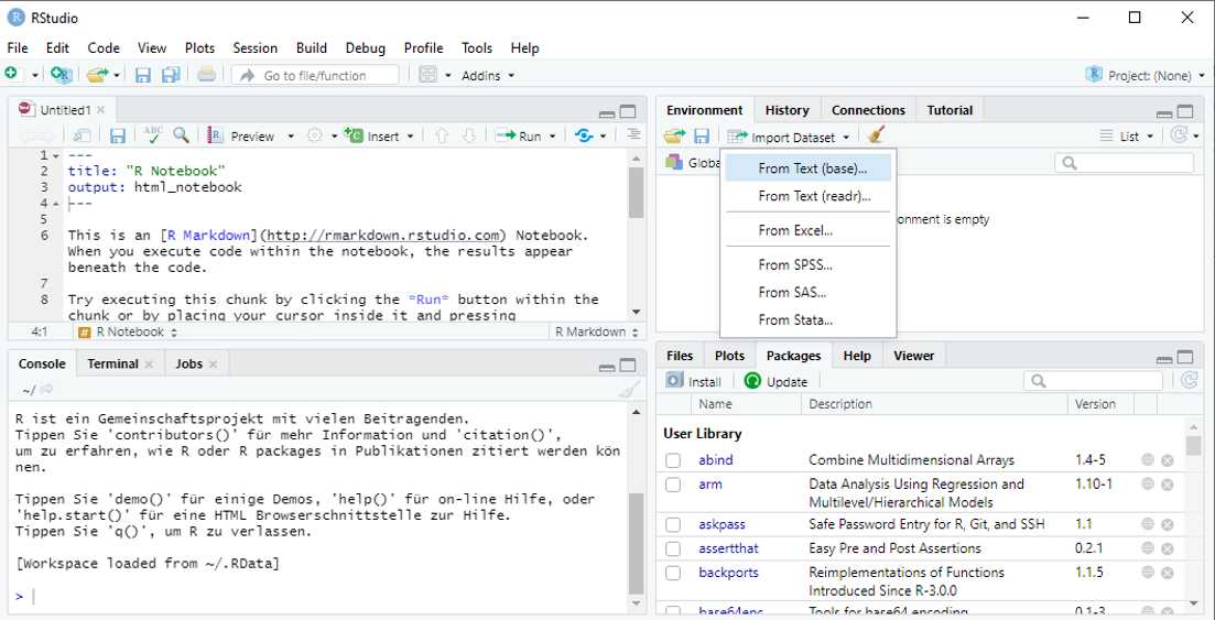
R offers quite a lot of options for importing external data. In RStudio the most comfortable way is via the “Import Dataset” dialog to be found in “Environment” ribbon of the right-upper pane:
 When importing data from text files (like .txt or .csv) it is recommended to use the
 readr package. Make sure that the proper options are selected to identify texts, columns, header etc.
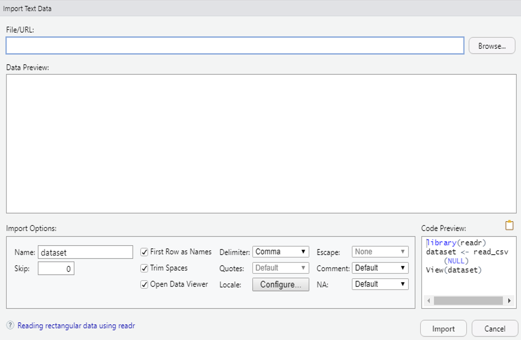
Take care of the font encoding as well as the data type inherited for each column. Best check the resulting data object not only as a whole, but also columnwise. Particularly, take care of columns with text as R has a tendency to convert text columns automatically into factors.
3.5 Exercises
- Calculate the outer product of two vectors (without
outer()). - Define a function that calculates the trace of a matrix.
- Create a vector containing the first 100 Fibonacci numbers.
- Create a matrix containing all binomial coefficients up to \(n=50\).
- Create a list containing
- a vector of 5 small letters
- a vector of 5 capital letters
- a vector of 5 random numbers
- Try to convert the matrix into a data frame.
- Create a matrix with dimension \(4\times 4\) and fill it with random numbers (Hint: Check out the functions
sample(),runif()andrnorm()). - For the matrix generated in task 6, check whether its invertable.
- For the matrix generated in task 6, check whether \(a_{ij} = a_{ji}\) holds.
- For the matrix generated in task 6, alter it such that \(a_{ij} = a_{ji}\) holds and set the diagonal elements to one.
- Write a function that checks for given matrix, whether
- its invertible
- \(a_{ij} = a_{ji}\) holds
- the diagonal elements are one.
- Additionally, calculate the matrix’ column sums and return all information in list of results.