Chapter 7 Optimization in R
There are a lot of optimization routines implemented in R. Most multi-purpose optimization routines in R are dedicated to continuous optimization as this is most often encountered in statistics. Additionally, also constrained optimization problems appear which are notoriously difficult to solve in their most general form. The following table shows an overview over some popular optimization routines in R. A comprehensive overview can be found here.
| type of objective func. | variables | constraints | package | function |
|---|---|---|---|---|
| general | 1, cont. | none | built-in | optimize() |
| general | \(n\), cont. | boxed | built-in | optim() |
| general | \(n\), cont. | boxed | optimx |
optimx() |
| general | \(n\), cont. | linear | built-in | constrOptim() |
| linear | \(n\), cont. | linear | lpSolve |
lp() |
| linear | \(n\), cont., int., bin. | linear | Rglpk |
Rglpk_solve_LP() |
| linear | \(n\), cont., int., bin. | linear | Rsymphony |
Rsymphony_solve_LP() |
| quad. | \(n\), cont. | linear | quadprog |
solve.QP() |
| general | \(n\), cont. | general | nloptr |
nloptr() |
| general | \(n\), cont. | general | Rsolnp |
solnp() |
7.1 Continuous optimization with optim
For unconstrained (or at most box-constraint) general prupose optimization, R offers the built-in function optim() which is extended by the optimx() function. The syntax of both functions is identical: optim(par = <initial parameter>, fn = <obj. function>, method = <opt. routine>). The first argument of the function to be optimized must be the vector (or scalar) to be optimized over and should return a scalar (i.e. the objective value). Some optimization routines also allow Inf or NA as returned values, but some require finite values always. Additionally, upper and lower values for the parameters can be set by option lower = <vector of lower bounds> and upper = <vector of upper bounds>. In this case, method = "L-BFGS-B" must be selected. By default, optim() and optimx() minimize the objective function.
# one-dimensional optimization
fn.poly <- function(x) 0.01 * x^3 + 2* x^2 + 1 * x + 4  # define a polynomial function
optim(par = 1, fn = fn.poly, method = "BFGS")    # one result list
optimx(par = 1, fn = fn.poly, method = c("Brent", "CG", "BFGS", "bobyqa", "nlm")) # and comparison of alternative methods
As an example for 2-dimensional optimization, the continuous location planning problem with Manhattan metric is considered:
\[\min\limits_{(u,v) \in \mathbb R^2} \rightarrow \sum_{i \in \mathcal{C} } a_i \cdot (|x_i - u| + |y_i - v|)\]
The weighted Manhattan distance function introduced before also handles vectors. So, we need to adapt this function only slightly:
loc.mh <- function(loc, a, x, y) sum(a * (abs(x - loc[1]) + abs(y - loc[2]) ) )
n <- 100
a.vec <- sample(1:100, size = n)    # sample weights for each point/customer
x.vec <- rnorm(n)                   # sample x coordinates
y.vec <- rnorm(n)                   # sample y coordinates
res <- optim(par = c(0,0), fn = loc.mh, method = "BFGS", a = a.vec, x = x.vec , y= y.vec)
# optimal location should be close to (0,0)
The corresponding solution can de plotted as follows (sizes of customer points are proportional to their weights \(a_i\)).
library(grDevices)        # package for generating color gradients
# generate grid of potential locations
emat <- expand.grid(seq(-3,3, length.out = 100), seq(-3,3, length.out = 100))
# list with grid point coordinates
plist <- list(x = seq(-3,3, length.out = 100), y = seq(-3,3, length.out = 100))
# evaluate objective function at each potential location
z.vec <- apply(emat, 1, function(x) loc.mh(x, a = a.vec, x = x.vec, y = y.vec))
# generate color vector --> assigns a color between green and red depending on the objective value
col.vec <- colorRamp(c("green","orange","red"))( (z.vec-min(z.vec))/(max(z.vec)) )
# recode color vector to RGB code
col.vec <- rgb(col.vec[,1],col.vec[,2],col.vec[,3], maxColorValue = 255)
# create plot
par(mar =c(4,4,0.3,0.3))
plot(emat, xlim=c(-3,3), ylim=c(-3,3), xlab="x", ylab="y", col = col.vec, pch = 15, asp = 1, xaxs = "i", yaxs = "i", cex = 1.5)
points(x.vec, y.vec, pch =20 , cex = log(a.vec)/2)
points(rbind(res$par,res$par), pch =17 , cex = 2, col="blue")
contour(plist, z= matrix(z.vec, ncol=100) , add= TRUE)
legend("topleft", bty="n", legend=c("customer","center"), col=c("black","blue"), pch = c(20,17), bg = "yellow", cex = 1.5)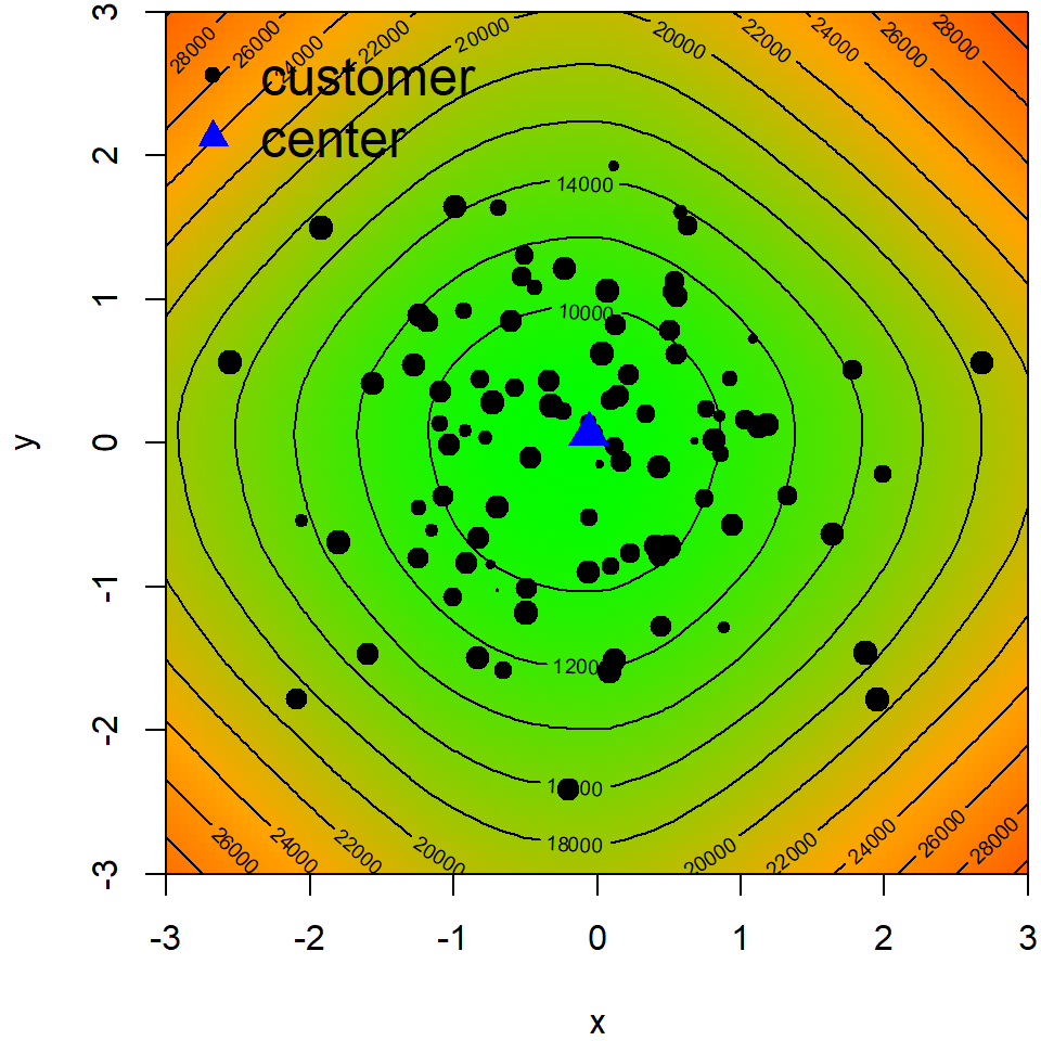
Figure 7.1: Value of objective function, customer points and optimal center
Exercise 1: Formulate the Steiner-Weber model (i.e., the continuous location planning problem with Euclidean distance metric) and solve it with
optim().
Exercise 2: Formulate the Newsvendor model \[Z(q) = \int_0^q{c_o \cdot (q-x) \cdot f(x, \mu, \sigma) \mathrm{d} x } + \int_q^\infty {c_u\cdot (x-q) \cdot f(x, \mu, \sigma) \mathrm{d} x }\] and use
optim()to find the optimal order quantity. Compare the optimal solution found byoptim()with the theoretical optimum.
7.2 Mixed-integer linear optimization with GLPK
7.2.1 Generic formulation of MILP models
Mixed-integer linear optimization problems (MILP) are characterized by linear objective functions and constraints w.r.t. the decision variables. However, some or all decision variables are integer and/or binary variables. In general, the canonical form of an MILP can be written as
\[ \min\limits_{ \mathbf{x}, \mathbf{y}, \mathbf{z}} \rightarrow \mathbf{c}_x^T \cdot \mathbf{x} + \mathbf{c}_y^T \cdot \mathbf{y} + \mathbf{c}_z^T \cdot \mathbf{z}\]
\[\begin{align} \mathbf{A}_x \cdot \mathbf{x} + \mathbf{A}_y \cdot \mathbf{y} + \mathbf{A}_z \cdot \mathbf{z} & \leq \mathbf{b} \\ \mathbf{x} & \in \mathbb{R} \\ \mathbf{y} & \in \mathbb{Z} \\ \mathbf{z} & \in \{0,1\} \\ \end{align}\]
Hence, a MILP basically consists of four parts:
- coefficient vector \(c = (c_x, c_y, c_z)\)
- constraint matrix \(A = (A_x,A_y,A_z)\)
- right-hand side vector \(\mathbf{b}\)
- direction of the constraints
- the domain declarations of the decision variables.
These five components are to be specified when a MILP is solved with R. In case, there are only continuous variables (i.e., a linear program), no domain declarations are necessary.
As an example, the dynamic lot-sizing problem or Wagner-Whitin model is considered where \(c_o\) is the ordering cost rate, \(c_h\) is the stock holding cost rate, and \(d_t\) denotes the demand in period \(t\). It is to decide whether to place an order in period \(t\) (i.e., \(y_t\) is 1 or 0), the corresponding order quantity (\(q_t\)), and the stock level \(l_t\). The MILP can be formulated compactly as: \[ \min\limits_{ l_t, q_t, y_t} \rightarrow \sum_{t = 1}^{T} \left(c_o \cdot y_t + c_h \cdot l_t \right)\]
\[\begin{align} l_{t-1} - l_t + q_t & = d_t & t = 1,...,T \\ q_t - M \cdot y_t & \leq 0 & t = 1,...,T \\ l_t & = 0 & t \in \{0,T\}\\ q_t, l_t & \geq 0 & t = 1,...,T\\ y_t & \in \{0,1\} & t = 1,...,T \\ \end{align}\]
7.2.2 Extensive model formulation
For \(T = 3\) periods, the canonical form of the Wagner-Whitin model consists of a vector of decision variables with 10 elements \(\mathbf x = (l_0,...,l_3,q_1,....,q_3,y_1,...,y_3)\). The vector of objective parameters is \(\mathbf c = (\underbrace{c_h,...,c_h}_{4},\underbrace{0,...,0}_{3},\underbrace{c_o,...,c_o}_{3})\). There are \(2 \cdot T + 2 = 8\) constraints. Thus, the right-hand side vector \(\mathbf b = (\underbrace{d_1,...,d_3}_{3},\underbrace{0,...,0}_{5})\). Correspondingly, the constraint matrix \(\mathbf A\) has dimension \(8 \times 10\) and looks as follows:
\[ \mathbf A = \left[ \begin{array}{*{10}{r}} 1 & -1 & 0 & 0 & 1 & 0 & 0 & 0 & 0 & 0 \\ 0 & 1 & -1 & 0 & 0 & 1 & 0 & 0 & 0 & 0 \\ 0 & 0 & 1 & -1 & 0 & 0 & 1 & 0 & 0 & 0 \\ 0 & 0 & 0 & 0 & 1 & 0 & 0 & -M & 0 & 0 \\ 0 & 0 & 0 & 0 & 0 & 1 & 0 & 0 & -M & 0 \\ 0 & 0 & 0 & 0 & 0 & 0 & 1 & 0 & 0 & -M \\ 1 & 0 & 0 & 0 & 0 & 0 & 0 & 0 & 0 & 0 \\ 0 & 0 & 0 & 1 & 0 & 0 & 0 & 0 & 0 & 0 \\ \end{array} \right] \] Thus, in R a dynamic lot-sizing problem can be formulated as follows
library(Rglpk)                      # load solver package
n <- 6                              # number of periods
co <- 50                            # ordering cost rate
ch <- 0.1                           # holding cost rate
d.vec <- round(rnorm(n, mean = 100, sd = 20))   # sample demand from normal distribution with mean 100 and sd 20
bigM <- sum(d.vec)                  # set big M
x.vec <- numeric(3*n + 1)           # initialize decision variables
b.vec <- c(d.vec, rep(0, n + 2))    # right-hand side vector
c.vec <- c(rep(ch, n+1), rep(0, n), rep(co, n))    # objective coefficient vector
const.vec <- c(rep("==", n), rep("<=", n) , rep("==", 2))    # vector with constraint directions
vtype.vec <- c(rep("C",n + 1), rep("C",n), rep("B",n))       # vector with variable types ("C" continuous,"I" integer, "B" binary )

A.mat <- matrix(0, ncol = 3*n + 1, nrow = 2*n+2)    # initialize constraint matrix
# write coefficient in first n rows (inventory constraints)
for(i in 1:n){
  A.mat[i,i]   <- 1         # coefficint for l_{t-1}
  A.mat[i,i+1] <- -1        # coefficint for l_{t}
  A.mat[i,n + 1 + i] <- 1   # coefficint for q_{t}
}
# write coefficient in rows (n+1):(2*n) (ordering constraints)
for(i in (n+1):(2*n)){
  A.mat[i,i+1] <- 1             # coefficint for q_{t}
  A.mat[i,n + 1 + i] <- -bigM   # coefficint for y_{t}
}
# write coefficient in last two rows (inventory inititialization)
  A.mat[nrow(A.mat)-1,1] <- 1    # coefficint for i_{0}
  A.mat[nrow(A.mat),n+1] <- 1    # coefficint for i_{T}

  A.mat

  # solve MILP
  sol <- Rglpk_solve_LP(obj = c.vec, mat = A.mat, dir = const.vec, rhs = b.vec, types = vtype.vec)
  # list with solution and demand
  list( l = sol$solution[1:(n+1)],         # inventory levels
        q = sol$solution[(n+2):(2*n+1)],   # order quantities
        y = tail(sol$solution, n),         # order indicators
        d = d.vec )                        # demand
By default, most solvers assume that decision variables are non-negative. Thus, in the example above,it is not necessary to add \(l_t \geq 0\) and \(q_t \geq 0\) to the constraint matrix \(\mathbf A\). Nonetheless, this should be checked by taking a look at the solver function’s help page.
Partiularly for larger MILPs the constraint matrices quickly become quite large. However, most entries are 0. Therefore, it is convenient to use sparse matrices. Sparse matrices are matrices where only non-zero entries are explicitly defined by there “coordinates” in the matrix (i.e. row and column index) and their value. In R one can use sparseMatrix() from the Matrix package to create such a matrix. The syntax to create a sparse matrix is sparseMatrix(i = <vector of row indices>, j = <vector of col. indices>, x = <vector of entries>, dims = <vector matrix dimensions>)
# assign names to decision vector
names(x.vec) <- c(paste("l", 0:n, sep=""), paste("q", 1:n, sep=""), paste("y", 1:n, sep=""))
nb.const <- 1         # initialize number of constraints
const.mat <- NULL     # initialize constraint data frame

# write inventory balance constraints
for(i in 1:n){
  tmp.ind.row <- rep(nb.const, 3)       # row index --> in each row, three non-zero entries
  tmp.ind.col <- c(i,                                             # l_{i-1}
                   which(names(x.vec) %in% paste("q",i, sep="")), # find index of q_i
                   i+1                                            # l_i
                  )
  tmp.const <- c(1,1,-1)                                          # assign coefficients
  const.mat <- rbind(const.mat, cbind(tmp.ind.row, tmp.ind.col, tmp.const)) # update constraint data frame
  nb.const <- 1 + nb.const                                        # update constraint index
  }

# write purchasing constraints
for(i in 1:n){
  tmp.ind.row <- rep(nb.const, 2)       # row index --> in each row, two non-zero entries
  tmp.ind.col <- c(which(names(x.vec) %in% paste("q",i, sep="")), # find index of q_i
                   which(names(x.vec) %in% paste("y",i, sep=""))  # find index of y_i
                  )
  tmp.const <- c(1,-bigM)                                          # assign coefficients
  const.mat <- rbind(const.mat, cbind(tmp.ind.row, tmp.ind.col, tmp.const)) # update constraint data frame
  nb.const <- 1 + nb.const                                        # update constraint index
  }

# add initialization constraints
const.mat <- rbind(const.mat,
                   cbind(nb.const  , 1  , 1), # l_0 = 0
                   cbind(nb.const+1, n+1, 1)) # l_T = 0

# write as sparse matrix
A.mat <- sparseMatrix(i = const.mat[,1], # vector of row indices
                      j = const.mat[,2], # vector of column indices
                      x = const.mat[,3], # vector of coefficients
                      dims = c(max(const.mat[,1]) , length(x.vec))) # matrix dimensions

# solve MILP
sol <- Rglpk_solve_LP(obj = c.vec, mat = A.mat, dir = const.vec, rhs = b.vec, types = vtype.vec)
# list with solution and demand --> same result as before
list( l = sol$solution[1:(n+1)],         # inventory levels
        q = sol$solution[(n+2):(2*n+1)],   # order quantities
        y = tail(sol$solution, n),         # order indicators
        d = d.vec )                        # demand
Exercise 3: Add an inventory capacity constrint to the Wagner-Whitin model and resolve it with
Rglpk.
Exercise 4: Solve the Transshipment Problem with
Rglpk: \[ \min\limits_{x_{ij}} \rightarrow \sum_{i \in \mathcal{V}_a }\sum_{j \in \mathcal{V}_t } c_{ij} \cdot x_{ij} + \sum_{j \in \mathcal{V}_t }\sum_{k \in \mathcal{V}_b } c_{jk} \cdot x_{jk} \] \[\begin{align} \sum_{j \in \mathcal{V}_t} x_{ij} & \leq a_i & \forall i \in \mathcal{V}_a \\ \sum_{j \in \mathcal{V}_t} x_{jk} & \geq b_k & \forall k \in \mathcal{V}_b \\ \sum_{i \in \mathcal{V}_a} x_{ij} & = \sum_{k \in \mathcal{V}_b} x_{jk} & \forall j \in \mathcal{V}_t \\ x_{ij} & \geq 0 \\ \end{align}\] where \(a_i\) is the maximum supply capacity of node \(i \in \mathcal{V}_a\), \(b_k\) denotes the demand of node \(j \in \mathcal{V}_b\), \(c_{ij/jk}\) are transport cost rates and \(x_{ij/jk}\) are shipment quantities.
How would you cope with transshipment capacities at nodes \(j \in \mathcal{V}_t\)?
How would you cope with fixed transshipment costs?
7.3 ROI: R Optimization Infrastructure
There are quite a lot of different optimization problems and associated R function where tailor-made solution algorithms are implemented. Although any optimization problem consists of objective function, variables, and constraints, there are numerous ways to formalize these components for submission to an optimization function in R. The package ROI attempts to provide a unified framework for seting up and solving generic optimization problems. An extensive description of the package can be found here.
library(ROI)            # load package
ROI_available_solvers() # check available solvers
ROI_installed_solvers() # check installed solvers
# install some new solvers
install.packages("ROI.plugin.quadprog")
install.packages("ROI.plugin.symphony")

ROI_installed_solvers() # check again
Commercial solvers for linear optimization problems are typically the most powerful solvers available but sometimes rather difficult to integrate into open-source project as they are proprieary software. Nonetheless, there are some workarounds for integrating Gurobi and CPLEX. Prerequisite is always that solver is already installed on your machine and the corresponding R-API is installed. For Gurobi the necessary API is bundled in an R package which is distributed with the software an zip-archive. Once Gurobi and the corresponding R package is installed, it can be registered and used as an ROI solver. Note that it might be necessary to install the ROI Gurobi plugin from the sources.
library(gurobi)         # load Gurobi package (to be found in the installation directory of Gurobi)
install.packages("ROI.plugin.gurobi", repos="http://R-Forge.R-project.org")
ROI_installed_solvers() # check again
To formulate an optimization problem, the function OP(objective, constraints, types, bounds) is used whereby the objective and constraint components are generated by creator functions. The types of variables are defined by a character vector of length \(n\) consisting of the characters “C”, “I” or “B” indicating continuous, integer or binary variables, respectively. Corresponsindgly, upper and lower bounds of the variables can be given as a named list consisting of two vectors of length \(n\) and named “lower” and “upper”.
For the objective function these creator functions are defined as follows:
| type | creator | description |
|---|---|---|
| function | F_objective(F,n,G,H,names) |
\(F(\mathbf x)\)…function to optimize, \(\mathbf x\)…vector of decision variables, \(G(\mathbf x)\)…gradient function (\(F'(\mathbf x)\), optional), \(H(\mathbf x)\)…Hessian function (\(F''(\mathbf x)\), optional), names…naming of variables |
| quadratic | Q_objective(Q,L,names) |
\(F(\mathbf x)= \frac{1}{2}\cdot \mathbf x^T \cdot \mathbf Q\cdot \mathbf x+ \mathbf x^T\cdot \mathbf l\), \(\mathbf Q\)…matrix (\(n\times n\)) with coefficients of quadratic terms, \(\mathbf l\)… vector of coefficients for linear terms, names…naming of variables |
| linear | L_objective(L,names) |
\(F(\mathbf x)= \mathbf x^T\cdot \mathbf l\), \(\mathbf l\)… vector of coefficients for linear terms, names…naming of variables |
The second component of optimization problems are the constraints. In general, the constraints consist of the left-hand side which depends on the decision variables \(x\), the right-hand side vector (\(\mathbf{b}\), rhs), and the direction vector (dir), e.g. \(lhs(\mathbf{x})\leq \mathbf{b}\). The left-hand side is created in a similar way as the objective function using the following creators
| type | creator | description |
|---|---|---|
| function | F_constraint(F,dir,rhs,names) |
\(F\)…list of functions with \(F=\left\{f_i(\mathbf x) \right\}\) such that \(f_i(\mathbf x) \leq b_i\) |
| quadratic | Q_constraint(Q,L,dir,rhs,names) |
left-hand side: \(\frac{1}{2}\cdot \mathbf x^T \cdot \mathbf Q\cdot \mathbf x+ \mathbf x^T\cdot \mathbf L\) with \(\mathbf Q\)…list of \(n\times n\)-matrices with coefficients of quadratic terms, \(\mathbf L\)…matrix of coefficients for linear terms |
| linear | L_constraint(L,dir,rhs,names) |
left-hand side: \(\mathbf x^T\cdot \mathbf L\), \(\mathbf L\)…matrix of linear coefficients |
The following example solves the continuous location planning problem via ROI:
n <- 100
a.vec <- sample(1:100, size = n)    # sample weights for each point/customer
x.vec <- rnorm(n)                   # sample x coordinates
y.vec <- rnorm(n)                   # sample y coordinates

copt <- OP(
  objective = F_objective(F = function(loc) sum(a.vec * (abs(x.vec - loc[1]) + abs(y.vec - loc[2]) ) ), n = 2),
  types = rep("C", 2),
  bounds = V_bound(ub = rep(Inf, 2), lb = rep(-Inf, 2))
)

copt_sol <- ROI_solve(copt, start = c(0,0))         # solve the problem
copt_sol$solution                                   # obtain solution
copt_sol$objval                                     # objective value
To change the problem, an already existing optimization problem can be updated componentwise:
# change objective function - inverted weights 1/a
objective(copt) <- F_objective(F = function(loc) sum( 1/a.vec * (abs(x.vec - loc[1]) + abs(y.vec - loc[2]) ) ), n = 2)

copt_sol <- ROI_solve(copt, start = c(0,0))         # solve the problem
copt_sol$solution                                   # obtain solution
copt_sol$objval                                     # objective value
Exercise 5: Change the problem by adding constraints that prohibit the center to be closer than 0.5 distance units to any point.
Exercise 6: Formulate the Newsvendor model with \(\beta\) service level restriction with the
ROIframework.
Similarly, the ROI can be used to solve mixed-integer problems. Consider the following linear assignment problem assigning \(n\) elements to \(n\) rooms in a cost-minimal way:
\[min \rightarrow \sum_{i,j =1}^n x_{ij} \cdot c_{ij}\]
subject to
\[\begin{align}
\sum_{i=1}^n x_{ij} &= 1 & \forall j = 1,...,n\\
\sum_{j=1}^n x_{ij} &= 1 & \forall i = 1,...,n\\
x_{ij} & \in \left\{0,1\right\}
\end{align}\]
In the extensive ILP formulation, the decision vector is defined as \(\mathbf{x} = (x_{11},x_{12},...,x_{1n},x_{21},...,x_{2n},...,x_{nn})\). For a linear assignment problem with 3 rooms/elements, the constraint matrix is constructs as
\[
\mathbf A = \left[
\begin{array}{*{10}{r}}
1 & 0 & 0 & 1 & 0 & 0 & 1 & 0 & 0 \\
0 & 1 & 0 & 0 & 1 & 0 & 0 & 1 & 0 \\
0 & 0 & 1 & 0 & 0 & 1 & 0 & 0 & 1 \\
1 & 1 & 1 & 0 & 0 & 0 & 0 & 0 & 0 \\
0 & 0 & 0 & 1 & 1 & 1 & 0 & 0 & 0 \\
0 & 0 & 0 & 0 & 0 & 0 & 1 & 1 & 1 \\
\end{array}
\right]
\]
Thus, a linear assignment problem can be formulated via ROI as follows:
# create problem dimension
n <- 10
# create cost vector
c.vec <- rpois(n^2, 100)    # sample costs from Poisson distribution with mean 100
# create empty constraint matrix
L.mat <- matrix(0, ncol = n^2, nrow = 2*n)
# first n rows
L.mat[1:n,] <- do.call(cbind, lapply(1:n, function(x) diag(n)))
# last n rows
L.mat[(n+1):(2*n),] <- t(sapply(1:n, function(x) c(rep(0,(x-1)*n), rep(1,n),rep(0,(n-x)*n) )))

# create optimization problem
copt <- OP(
  objective = L_objective(L = c.vec),
  constraints = L_constraint(L = L.mat, dir = rep("==", 2*n), rhs = rep(1, 2*n)),
  types = rep("B", n^2)
)

copt_sol <- ROI_solve(copt)         # solve the problem
copt_sol$solution                   # obtain solution
copt_sol$objval                     # objective value

# display solution in matrix form
sol.mat <- matrix(copt_sol$solution, ncol = n)
# check first set of constraints
colSums(sol.mat)                    # all column sums equal to 1?
# check second set of constraints
rowSums(sol.mat)                    # all row sums equal to 1?
# check objective
sum(sol.mat * matrix(c.vec, ncol = n))
Exercise 7: Formulate the constraint matrix
Las a sparse matrix.
Exercise 8: Implement the quadratic assignment problem with
ROI. Can you reuse parts of the linear assignment problem?
7.4 Algebraic model formulation with ompr
Algebraic model formulations allow one to pass MILPs in math-like way to a solver. Algebraic modelling languages are usually used to formulate large and/or complex optimization problems. Thus, commercial solvers often provide a tailored algebraic programming language like ILOG OPL or A/GMPL. The package ompr provides a similar access for modelling MILPs in a algebraic way. The package uses the ROI framework for accessing MILP solvers. The application of the package is illustrated by modelling the well-known travelling salesman problem (TSP).
Given a set of nodes \(\mathcal{N}\) with \(n = |\mathcal{N}|\) and pairwise distances \(d_{ij}\) between any pair of nodes (\(i,j \in \mathcal{N}\)), the TSP is to find the shortest tour which visits all nodes and returns to the origin. The following code snippet generates a set f nodes and displays the nodes
library(ggplot2)
# set number of nodes
n <- 10
# sample node coordinates
cities <- data.frame(id = 1:n, x = runif(n), y = runif(n))
# plot nodes
ggplot(cities, aes(x, y)) + geom_point() 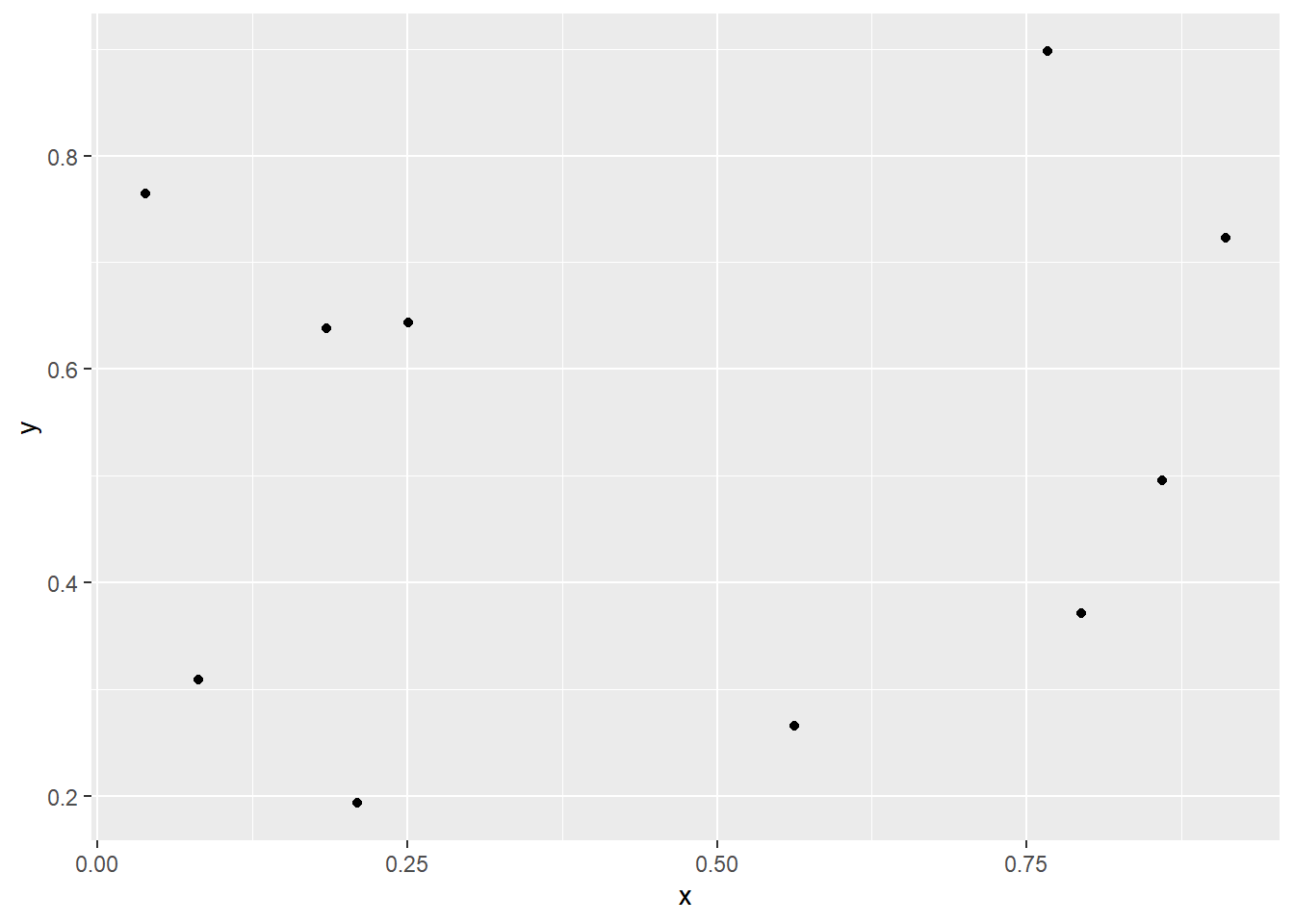
To formulate the TSP as a ILP, various formulations are available. Here, a simple formulation to avoid subtours is proposed: the Miller-Tucker-Zemlin formulation.
\[\min \rightarrow \sum_{i=1}^n \sum_{j=1}^n d_{ij} \cdot x_{ij}\]
\[\begin{align} \sum_{i \in \mathcal{N}: i\neq j} x_{ij} & = 1 & \forall j \in \mathcal{N} \\ \sum_{j \in \mathcal{N}: j\neq i} x_{ij} & = 1 & \forall i \in \mathcal{N} \\ u_j & \geq u_i + 1 - n \cdot (1-x_{ij}) & \forall i,j \in \mathcal{N}, i \neq j, i,j>1 \\ u_1 & = 1 & \\ u_i & \in \left[2,n\right] & \forall i \in \mathcal{N}, i>1\\ x_{ii} & = 0 & \forall i \in \mathcal{N} \\ x_{ij} & \in \left\{0,1\right\} & \forall i,j \in \mathcal{N} \end{align}\]
Setting up the ILP with ompr uses so-called pipes. Piping is an instrument to simplify code in R. Typically, more complex analyses in R often call multiple function subsequently whereby each function produces intermediate results which are passed (sometimes after some alterations) to the next function, i.e. code of the form \(x \rightarrow f(x) \rightarrow g(f(x))\). In case, there is such a sequence of functions instead of writing g(f(x)) the equivalent pipe is x %>% f %>% g, e.g. log(sqrt(x=2)) is equivalent to x %>% sqrt %>% log. The piping operaor is part of dplyr package, see here for an introduciton and some more advanced piping methods.
For setting up a MILP, the MIPModel() function is fed by piping constraints, variables, and objective functions using helper functions of the form add_<object>() and set_<object>(). The objects containing the data which are referred to in the helper functions should exist in the workspace before the MIPModel() function is called as this functions creates the extensive model formulation. The helper expressions like add_variable(<expr>, <quant>) consist of two parts: the expression and a quntifier. Thereby, the expression must be vectorized. I.e., the expression must accept vector inputs and return a vector of the same length. In the TSP case, the access to the distance matrix must be vectorized as follows.
library(ompr)
library(dplyr)
library(ompr.roi)
library(ROI.plugin.glpk)

distance <- as.matrix(dist(cities[,c("x","y")]))       # calculate distances
# create vectorized function for accessing distance values
dist_fun <- function(i, j) {
  vapply(seq_along(i), function(k) distance[i[k], j[k]], numeric(1L))
}
# compare results: retain distance of arcs (1,2), (2,3), and (3,4)
distance[c(1,2,3), c(2,3,4)]
dist_fun(c(1,2,3), c(2,3,4))
Exercise 9: The function for accessing the distances is obtained from here. Try to formulate a more compact
dist_fun().
Now, the TSP can be modelled as follows:
model <- MIPModel() %>%
  # create decision variable that is 1 iff we travel from node i to j
  add_variable(x[i, j], i = 1:n, j = 1:n, type = "integer", lb = 0, ub = 1) %>%
  # a helper variable for the MTZ formulation of the tsp
  add_variable(u[i], i = 1:n, lb = 1, ub = n) %>%
  # minimize travel distance
  set_objective(sum_expr(dist_fun(i, j) * x[i, j], i = 1:n, j = 1:n), "min") %>%
  # leave each node
  add_constraint(sum_expr(x[i, j], j = 1:n) == 1, i = 1:n) %>%
  # visit each node
  add_constraint(sum_expr(x[i, j], i = 1:n) == 1, j = 1:n) %>%
  # ensure no subtours (arc constraints)
  add_constraint(u[1] == 1) %>%
  add_constraint(u[j] >= u[i] + 1 - n * (1 - x[i, j]), i = 1:n, j = 2:n) %>%
  # exclude self-cycles
  set_bounds(x[i, i], ub = 0, i = 1:n)

# solve model with GLPK
result <- solve_model(model, with_ROI(solver = "glpk", verbose = TRUE))

# obtain solution
solution <- get_solution(result, x[i, j]) %>%
  filter(value > 0)
Note that the model variables (in the TSPexample x and u) should not exist in the workspace before setting up the MILP model. Otherwise, a warning will be produced.
The solution can be displayed as a graph with the corresponding tour.
# use auxiliary u variables to reorder the data frame of nodes
ggplot(cities[c(order(get_solution(result, u[i])$value),1),], aes(x, y)) +
  geom_point() +
  geom_text(aes(label=id),hjust=0, vjust=0) +
  geom_path() +
  ggtitle(paste0("Total cost: ", round(objective_value(result), 2)))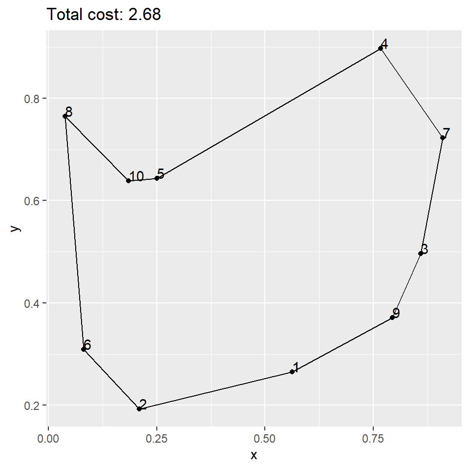
Figure 7.2: Optimal TSP tour
Exercise 10: Implement and solve the Wagner-Whithin modell introduced above with
ompr.